Classification, a cornerstone of supervised learning, empowers us to achieve this very goal. This comprehensive guide delves into the world of classification in Python, equipping you to build models that can accurately predict the category to which a new, unseen data point belongs.
What is Classification?
Classification is a supervised machine learning technique that aims to learn a mapping function from input features to a set of predefined categories or classes. Here’s how it works:
- Training Data: We provide the model with labeled data, where each data point consists of features (attributes) and a corresponding class label.
- Model Training: The model learns the relationship between features and class labels by analyzing the training data.
- Prediction: Once trained, the model can predict the class label for a new, unseen data point based on its features.
Classification Applications:
Classification finds applications in diverse domains:
- Spam Filtering: Classifying emails as spam or not-spam.
- Image Recognition: Categorizing images into objects like cars, dogs, or landscapes.
- Fraud Detection: Identifying fraudulent transactions based on financial data.
- Sentiment Analysis: Classifying text into positive, negative, or neutral sentiment.
- Customer Segmentation: Grouping customers based on purchase history or demographics.
Common Classification Algorithms:
Logistic Regression:
A popular technique for binary classification (two classes) that models the probability of a data point belonging to a specific class.
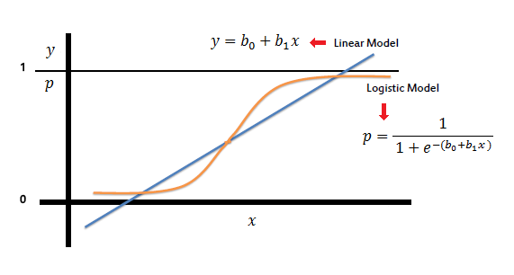
What is Logistic Regression
Logistic Regression predicts the binary outcome from a linear combination of one or more predictor (independent) variables. It is also known as the logit model. It works when depending on a variable is binary. And independent variable is independent of each other.
Types Of Logistic Regression:
- Binary logistic regression: It has only two possibilities depending on the variable. Example- win or loss
- Multinomial logistic regression: three or more nominal categories. Example- eye, hair, skin colour.
- Ordinal logistic regression: three or more ordinal categories, ordinal means category in an order format. Example- user ratings (1-10).
#create Logistic Regression model
logmodel = LogisticRegression()
logmodel.fit(X_train, y_train)
#predict on test data
predictions = logmodel.predict(X_test)
#confusion matrix, accurarcy
print(classification_report(y_test, predictions))
print(confusion_matrix(y_test, predictions))
print(accuracy_score(y_test, predictions))
Full Code: click Hear
K-Nearest Neighbors (KNN):
A simple algorithm that classifies a data point based on the majority class of its K nearest neighbors in the training data.
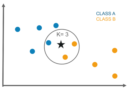
What is K-NN algorithm?
KNN is a lazy and non-parametric algorithm. This means creating boundaries to classify the point (data). When newly data points come in, try to predict that to the nearest of the boundary line called a non-parametric. There is no or minimal training phase, because of which the training phase is pretty fast. The K-nearest neighbour algorithm uses training data during the testing phase. K-nearest neighbour sort form is K-NN.
#make model
knn = KNeighborsClassifier(n_neighbors=7)
knn.fit(X_train, y_train)
#see score
print(knn.score(X_test, y_test))
Full Code : Click hear
Decision Trees:
A tree-like structure that classifies data points by asking a series of questions about their features.
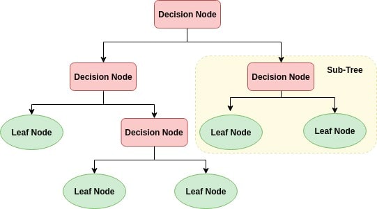
What is Decision Tree Classification algorithm?
Decision Tree is an algorithm of supervised machine learning. Tree-like structure As A Root Node, Internal Node And Leaf Node in a decision tree. It starts at the Root Node, the decision tree’s first node. The data set is split based on Root Node. Again, nodes are selected to split the already split data further. This process of splitting the data goes on till we get leaf nodes, which are nothing but the classification labels.
Decision Tree captures Non-linear patterns, visualizes and interprets without any assumptions. It is also used in feature engineering. The data set is biased when an imbalanced dataset.
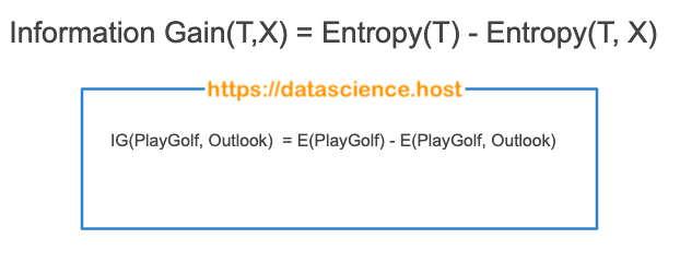
Information Gain: The process of selecting Root Nodes and Internal Nodes uses the statistical measure called Gain. Gain is the reduction of this uncertainty measure. Gain for any column calculated by differencing the Information Gain of a dataset to a variable from the Information Gain of the entire dataset.
Gini index: Gini is a metric for deciding how to split a Decision Tree. If select two items from a population at random, they must be of the same class and probability. The population is pure. Then it is denoted by 1. Gini measurement is the probability of a random sample being classified correctly if you randomly pick a label according to the distribution in the branch.
Entropy: Entropy is a probabilistic measure of uncertainty or impurity or calculates the lack of information when spilt the data. When a node is homogeneous, it is denoted by 0. this is desirable for a data scientist.
# Create Decision Tree classifer object
clf = DecisionTreeClassifier()
# Train Decision Tree Classifer
clf = clf.fit(X_train,y_train)
#Predict the response for test dataset
y_pred = clf.predict(X_test)
Full Code : Click Hear
Support Vector Machines (SVMs):
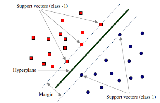
A powerful technique that finds a hyperplane that best separates data points of different classes.
What SVM?
Support vector machine (SVM) Classifier plots each data point in n-dimensional space with the value. It values each dimension being the value of a particular coordinate. Then, we perform classification to find the hyperplane that differentiates the classes well on SVM handle categorical and multiple continuous variables. Categorical variables have to be converted to numeric by creating dummy variables. Kernel, Regularization, Gamma And Margin tuning parameters mathematical computations that require numeric variables.
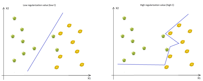
Regularization: Regularization parameters give a value for how to avoid misclassifying each training observation.
Margin: Margin is the separation line (Gap) to the closest class data points. The larger the margin width, the better the classification.
Kernel SVM
Kernel: transformations applied on input variables which separate non-separable data to separable data. In nonlinear separation, the problem helps to build a more accurate classifier.
There are 9 different kernel parameters: linear, nonlinear, polynomial, Gaussian kernel, Radial basis function (RBF), sigmoid, Laplace, Hyperbolic tangent And ANOVA.
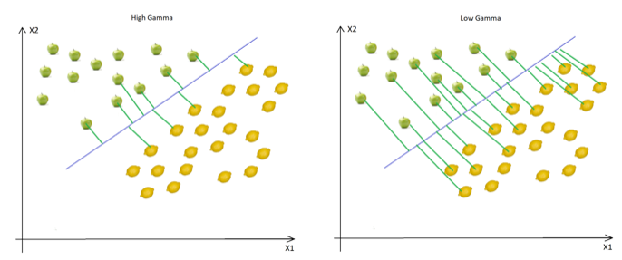
Gamma: Gamma is the kernel coefficient in the nonlinear kernel. Gamma is used for how far the impact of a single training example reaches: Example: RBF (Radial basis function), Polynomial, and Sigmoid. Higher values of Gamma will make the model more accurate, more complex, overfits and biased.
from sklearn import svm
#create a classifier
cls = svm.SVC(kernel="linear")
#train the model
cls.fit(X_train,y_train)
#predict the response
pred = cls.predict(X_test)
Full Code Link: Click Hear
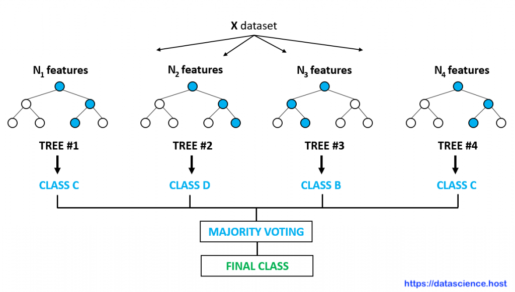
Random Forests:
An ensemble method that combines multiple decision trees for improved performance and robustness.
What is Random Forest Classification Algorithm?
Random Forest is an Algorithm of supervised machine learning. It Builds Multiple decision trees and randomly selects sample data and predicts. And compare all decision tree predictions also say voting method. Select the most contributing features and missing values using a Random forest classifier. It is slow in generating slow predictions. That’s why it is a time-consuming but highly accurate Algorithm. also well known as Bootstrap Aggregation And bagging Algorithm
#Create a Gaussian Classifier
clf=RandomForestClassifier(n_estimators=100)
#Train the model using the training
clf.fit(X_train,y_train)
y_pred=clf.predict(X_test)
Full Code : Click Hear
Naive Bayes
What is Naive Bayes algorithm?
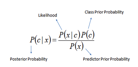
Naive Bayes is a classification algorithm based on Bayes Theorem with all independent (features) variables being independent and not related to each covariate (predictors). That’s why Naive Bayes call so ‘naive’.
Bayes Theorem finds the probability of an event occurring given the probability of another event that has already occurred. Mathematically it is given as P(A|B) = [P(B|A)P(A)]/P(B) where A & B are events. P(A|B) called Posterior Probability is the probability of event A(response) given that B(independent) has already occurred. P(B|A) is the likelihood of the training data, i.e., the probability of event B(independent) given that A(response) has already occurred. P(A) is the probability of the response variable, and P(B) is the probability of the training data or evidence.
# implement Model
ignb = GaussianNB()
pred_gnb = ignb.fit(Xtrain,ytrain).predict(Xtest)
#multinomial naive bayes
imnb = MultinomialNB()
pred_mnb = imnb.fit(Xtrain,ytrain).predict(Xtest)
Full Code: Click Hear
These are just a few examples, and the choice of algorithm depends on factors like data type, problem complexity, and desired performance.
Python to Code Examples for Classification Techniques
Let’s solidify our understanding with some code examples using popular Python libraries:
1. Logistic Regression with scikit-learn:
from sklearn.linear_model import LogisticRegression

# Load your labeled data (replace with your actual data)
X = ...  # Features
y = ...  # Class labels

# Create a LogisticRegression object
model = LogisticRegression()

# Train the model on the data
model.fit(X, y)

# Make predictions on a new data point (replace with your actual data)
new_data = ...

# Predict the class label for the new data point
predicted_label = model.predict(new_data.reshape(1, -1))

# Print the predicted label
print("Predicted class:", predicted_label[0])
This code demonstrates using Logistic Regression for binary classification with scikit-learn. We define a LogisticRegression object, train it on the labeled data, and then use the predict method to predict the class label for a new data point.
2. K-Nearest Neighbors (KNN) with scikit-learn:
from sklearn.neighbors import KNeighborsClassifier

# Load your labeled data (replace with your actual data)
X = ...  # Features
y = ...  # Class labels

# Define the number of neighbors (k)
k = 5

# Create a KNeighborsClassifier object
knn = KNeighborsClassifier(n_neighbors=k)

# Train the KNN model on the data
knn.fit(X, y)

# Make predictions on a new data point (replace with your actual data)
new_data = ...

# Predict the class label for the new data point
predicted_label = knn.predict(new_data.reshape(1, -1))

# Print the predicted label
print("Predicted class:", predicted_label[0])
This code snippet showcases KNN classification. We define the number of neighbors to consider (k) and create a KNeighborsClassifier object. The model is trained, and the predict method is used to make predictions for a new data point.
3. Decision Tree Classification with scikit-learn:
from sklearn.tree import DecisionTreeClassifier

# Load your labeled data (replace with your actual data)
X = ...  # Features
y = ...  # Class labels

# Create a DecisionTreeClassifier object with optional parameters
tree = DecisionTreeClassifier(criterion='gini', max_depth=3, random_state=42)

# Train the decision tree model on the data
tree.fit(X, y)

# Make predictions on a new data point (replace with your actual data)
new_data = ...

# Predict the class label for the new data point
predicted_label = tree.predict(new_data.reshape(1, -1))

# Print the predicted label
print("Predicted class:", predicted_label[0])

# Optionally, visualize the decision tree (requires graphviz)
from sklearn.tree import export_graphviz
import graphviz

dot_data = export_graphviz(tree, out_file=None,
                           filled=True, rounded=True,
                           special_characters=True, feature_names=X.columns)

graph = graphviz.Source(dot_data)
graph.render("decision_tree")  # Replace "decision_tree" with your desired filename
Use code with caution.content_copy
Explanation of Additions:
- Optional Parameters: The code now includes optional arguments for the
DecisionTreeClassifierconstructor:criterion: Specifies the splitting criterion used to create the decision tree (here, ‘gini’ for Gini impurity).max_depth: Limits the maximum depth of the tree, preventing overfitting (here, set to 3 for illustration).random_state: Sets a seed for random number generation, ensuring reproducibility (here, set to 42).
- Prediction: Similar to previous examples, the code predicts the class label for a new data point.
- Visualization (Optional): This section demonstrates how to visualize the decision tree using
graphviz. It requires thegraphvizlibrary to be installed. The code creates a DOT language representation of the tree and then usesgraphviz.Sourceto render it as a visual image file (e.g., “decision_tree.png”).
Remember to replace X, y, and new_data with your actual data before running the code.
Evaluation Metrics
- Evaluation Metrics: Classification models are evaluated using metrics like:
- Accuracy: The proportion of correctly classified data points.
- Precision: The proportion of true positives among predicted positives.
- Recall: The proportion of true positives identified by the model.
- F1-score: A harmonic mean of precision and recall, balancing both metrics.
These metrics provide insights into the performance of your classification model.
Considerations and Best Practices
Train-Test Split: Splitting your data into training and testing sets ensures the model doesn’t overfit to the training data. The training set is use to train the model, while the testing set is use to evaluate its performance on unseen data.
Hyperparameter Tuning: Many classification algorithms have hyperparameters that can be tune to improve performance. Techniques like grid search or random search can be employe to find the optimal hyperparameter settings.
Model Complexity: Striking a balance between model complexity and performance is crucial. Overly complex models can lead to overfitting, while underfitting models might not capture the underlying relationships in the data.
Error Analysis: Analyzing misclassified data points can provide valuable insights into potential issues with the model or the data. This can help refine your approach and improve future performance.
Conclusion
Classification in Python equips you with a powerful tool to automate decision-making by learning to categorize data points into predefined classes. By understanding different classification algorithms, their strengths and weaknesses, and best practices, you can effectively build models that unlock valuable insights from your data. Remember, the choice of algorithm, proper data handling, evaluation, and continuous improvement are all essential steps in achieving robust and accurate classification results. Embrace the power of classification to transform your data into actionable knowledge across various domains.pen_spark