Regression In Python

What Is Regression?

Regression is statistical processes for find relationship between depends variable and independent variables. depended variable also called as predict or outcome variable. independent variable also call as predictors, covariates, or features variable. independent may be one or more variables.

Regression analysis use for prediction, forecasting and analyse relationship between dependent and independent variable.

Simple Linear Regression

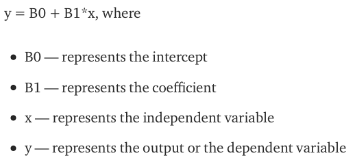
A model that Predict a linear relationship between the independent variable (x) and the depend (output) variable (y) called as Linear regression or linear model.

#import library
import numpy as np
import pandas as pd
import scipy.stats as stats
from sklearn.linear_model import LinearRegression
import matplotlib.pyplot as plt
#import data set
Emp_data = pd.read_csv("~/Downloads/Data Science/data set/emp_data.csv")
#spilt data set for independent and depend future
x = Emp_data.iloc[:, :-1].values 
y = Emp_data.iloc[:,-1:].values 
#qq plot
stats.probplot(Emp_data.Churn_out_rate, dist="norm", plot=plt)
plt.title("Normal Q-Q plot")
plt.show()
stats.probplot(Emp_data.Salary_hike, dist="norm", plot=plt)
plt.title("Normal Q-Q plot")
plt.show()
plt.plot(Emp_data.Churn_out_rate,Emp_data.Salary_hike) 
plt.show() 
#Multicollinearity check
corr = Emp_data.corr()
corr.style.background_gradient(cmap='coolwarm')
#create model
reg = LinearRegression()
#fit model
reg.fit(x,y)
print(reg.score(x, y)) 
#transform future for better accuracy
reg.fit(np.log(x),y)
print(reg.score(np.log(x), y)) 
reg.fit(np.log(x),np.log(y))
print(reg.score(np.log(x),np.log(y)))

GitHub Link : Click Hear

Linear Regression Assumptions :

Relationship : A must be linear relationship between independent and predict variables.

No Collinearity : Remove multicollinearity between predictors variables. because model difficult to predict which predictor variable are affect depend variable which not. independent variables depend from each other call multicollinearity

Auto correlations: No Residual Errors Dependent On Each Other. Most Of It is Occur in time series models because where the next instant is dependent on previous instant.

Heteroskedasticity : No Heteroskedasticity, in the scatter plot Should be clear pattern distribution of data called homoscedasticity.

Normal distribution: random variables should be normally distributed. This Is Check using Q-Q Plot.

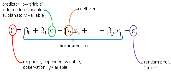
Multiple Linear Regression

Multiple linear regression is predict relationship between one continuous predict variable and two or more predictors variables. The predictors variables can be continuous or categorical. if categorical then need to convert them dummy variables.

#import libarary
import pandas as pd 
import numpy as np
import matplotlib.pyplot as pltfrom 
from sklearn.linear_model import LinearRegression
#read csv file
ComputerData = pd.read_csv("~/Downloads/Data Science/data set/Computer_Data.csv")
#Find Correlaton
corr = ComputerData.corr()
corr.style.background_gradient(cmap='coolwarm')
#split data using columan name
x = pd.DataFrame(ComputerData, columns = ['speed', 'hd', 'ram', 'screen', 'ads', 'trend'])
y = pd.DataFrame(ComputerData, columns = ['price'])
# Scatter plot between the variables along with histograms
import seaborn as sns
sns.pairplot(ComputerData)
# Preparing model                  
reg = LinearRegression()
reg.fit(x,y)
#check score
reg.score(x,y)

GitHub Link : Click Hear

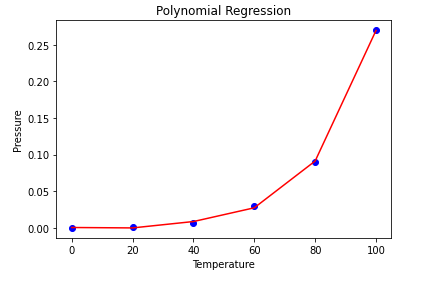
Polynomial Regression

Polynomial Regression: If (Y)Depened And (X)Indepened variable is correlated but relationship is not liner.

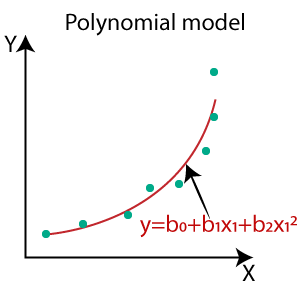
Broad range of function will be fit under it. but too sensitive to the outliers. The presence of one or two outliers within the data can seriously affect the results of the nonlinear analysis.Polynomial basically fits wide selection of curvature.

# Import libraries 
import numpy as np 
import matplotlib.pyplot as plt 
import pandas as pd 
from sklearn.preprocessing import PolynomialFeatures 
from sklearn.linear_model import LinearRegression 
# Import the dataset 
datas = pd.read_csv('~/Downloads/Data Science/data set/data.csv') 
datas 
X = pd.DataFrame(datas, columns = ['Temperature'])
y = pd.DataFrame(datas, columns = ['Pressure'])
# Fitting Linear Regression
lin = LinearRegression() 
lin.fit(X, y) 
# Fitting Polynomial Regression
poly = PolynomialFeatures(degree = 4) 
X_poly = poly.fit_transform(X) 
poly.fit(X_poly, y) 
lin2 = LinearRegression() 
lin2.fit(X_poly, y) 
# Visualise Linear Regression results 
plt.scatter(X, y, color = 'blue') 
plt.plot(X, lin.predict(X), color = 'red') 
plt.title('Linear Regression') 
plt.xlabel('Temperature') 
plt.ylabel('Pressure') 
plt.show() 
# Visualise Polynomial Regression results 
plt.scatter(X, y, color = 'blue') 
plt.plot(X, lin2.predict(poly.fit_transform(X)), color = 'red') 
plt.title('Polynomial Regression') 
plt.xlabel('Temperature') 
plt.ylabel('Pressure') 
plt.show() 

Github link: Click Hear

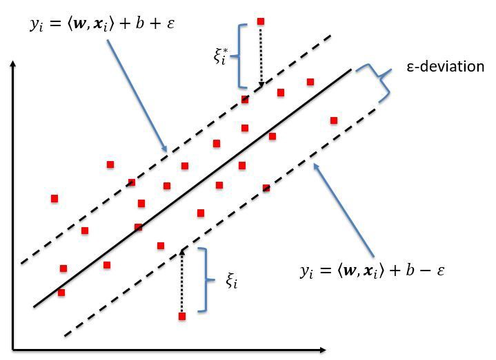
Support Vector Regression (SVR)

Support Vector regression is a part of Support vector machine that supports both linear and non-linear regression.

from sklearn.svm import SVR
regressor = SVR(kernel = 'rbf')
regressor.fit(X, y)
#predicte new value
y_pred = regressor.predict(6.5)
y_pred = sc_y.inverse_transform(y_pred) 
view raw

Github Link : Click Hear

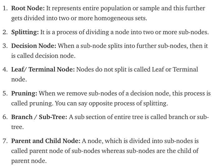
Decision Tree Regression

When Out Predicted Variable is continuous (real numbers) then applies Decision Tree Regression

# create a decisiontreeregressor model 
regressor = DecisionTreeRegressor(random_state = 0) 
# fit the regressor with X and Y data 
regressor.fit(X, y) 

Github Link : Click Hear

Random Forest Regression

A Random Forest is an ensemble technique. opposite to build a single decision tree. random forest build many decision trees. Then combine every decision tree output and give stable output. this technique called Bootstrap Aggregation also known as bagging.

# import the regressor 
from sklearn.ensemble import RandomForestRegressor 
# create regressor object 
regressor = RandomForestRegressor(n_estimators = 100, random_state = 0) 
# fit the regressor with x and y data 
regressor.fit(X, y) 

Github Code : Click Hear

Conclusion

When Predicted Variable is Should Be Continuous. if not then create dummy variable. in python most of NumPy, scikit-learn, and statsmodels library used.