R for data science

data science, the ability to manipulate, analyze, and visualize data effectively is paramount. R, a powerful open-source programming language, has emerged as a go-to tool for data scientists worldwide. This comprehensive guide explores the versatility of R for data science, its features, and its applications across various domains.

What is R?

R is a free, open-source programming language and software environment designed specifically for statistical computing and graphics. Initially developed in the early 1990s, R has since gained widespread popularity among data scientists, statisticians, and researchers due to its extensive capabilities in data manipulation, visualization, and statistical modeling.

Why Choose R for Data Science?

1. Freely Available and Customizable: As an open-source language, R is freely available and customizable, making it an attractive choice for individuals and organizations alike.
2. Efficient Data Wrangling: R’s data structures, such as data frames, provide efficient ways to handle and manipulate large datasets, enabling seamless data preprocessing and transformation.
3. Vast Library Ecosystem: With thousands of user-contributed packages, R offers a vast collection of tools and libraries for various data science tasks, including machine learning, text mining, and data visualization.
4. Reproducible and Collaborative: R’s ability to integrate code, data, and visualizations into a single document (using tools like R Markdown) facilitates reproducible research and collaborative work.
5. Active and Supportive Community: R benefits from a vibrant global community of developers, researchers, and enthusiasts who contribute to its growth and share knowledge.

Key Features of R for Data Science:

1. Data Wrangling with tidyverse: The tidyverse collection of packages, including dplyr and tidyr, provides a consistent and intuitive syntax for data manipulation and cleaning tasks.
2. Powerful Data Visualization: The ggplot2 package, based on the “Grammar of Graphics” concept, offers a flexible framework for creating high-quality visualizations, from simple plots to intricate statistical graphics.
3. Comprehensive Statistical Modeling: R’s comprehensive libraries, such as caret and mlr, enable a wide range of statistical modeling and machine learning techniques, from regression to deep learning.
4. Reproducible Reports: R Markdown allows users to create dynamic documents that combine code, text, and visualizations, facilitating collaborative work and reproducible research.
5. Integration with Other Tools: R seamlessly integrates with various data storage solutions, databases, and other programming languages like Python, enabling efficient data exchange and interoperability.

Applications of R in Data Science:

R finds applications across various domains, including but not limited to:

1. Finance and Banking: Analyzing financial data, risk modeling, and portfolio optimization.
2. Healthcare and Biostatistics: Clinical trials analysis, genomic data analysis, and epidemiological studies.
3. Marketing and Consumer Analytics: Customer segmentation, market basket analysis, and sentiment analysis.
4. Environmental Science: Ecological modeling, climate data analysis, and spatiotemporal data analysis.
5. Social Sciences: Survey analysis, experimental design, and behavioral data analysis.

Getting Started with R for Data Science:

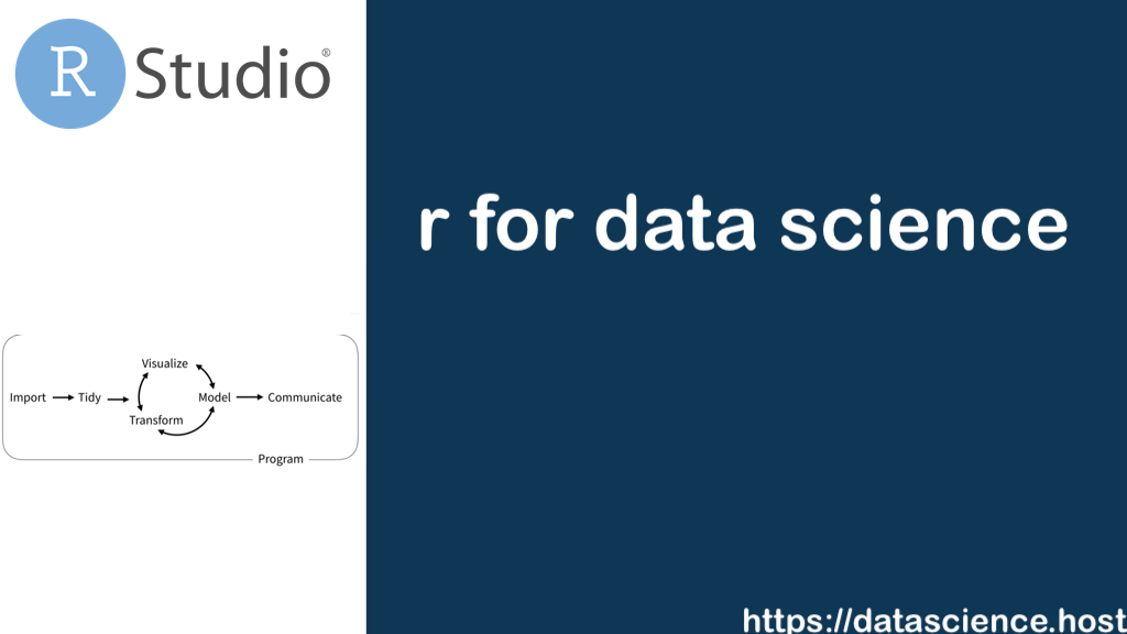
To begin your journey with R for data science, several resources are available. The book “R for Data Science” by Hadley Wickham and Garrett Grolemund, now in its 2nd edition, provides a solid foundation and practical examples for leveraging R’s capabilities. Additionally, online tutorials, interactive coding platforms like DataCamp and Coursera, and engaging with the active R community through forums, meetups, and conferences can provide invaluable support and networking opportunities.

Conclusion:

R has solidified its position as a powerful and versatile open-source programming language for data science. With its efficient data wrangling capabilities, extensive library ecosystem, and tools for reproducible research, R empowers data scientists to tackle complex projects across various domains. Whether you’re a seasoned data scientist or just starting your journey, embracing R can unlock the full potential of your data and drive impactful insights.