Clustering in Python

machine learning, where data reigns supreme, the ability to group similar data points together holds immense value. This is where clustering techniques come into play. This comprehensive guide delves into the world of clustering in Python, empowering you to uncover hidden structures within your data and organize it into meaningful groups, also known as clusters.

What is Clustering?

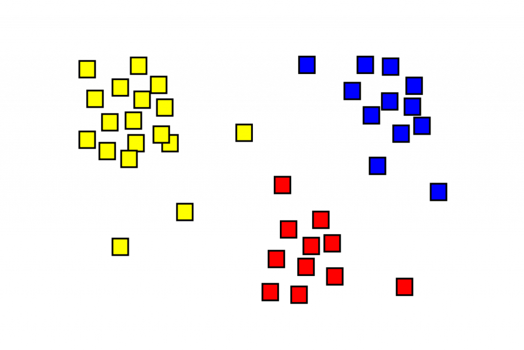
Clustering is an unsupervised learning technique that groups data points into clusters based on their similarity. Imagine a dataset containing information about different species of flowers. Clustering can group these flowers based on features like petal length, petal width, and color, revealing underlying patterns in the data. Here are some key benefits of clustering:

• Data Exploration and Visualization: Clustering helps identify natural groupings within data, aiding in data exploration and visualization. By visualizing the clusters, you can gain a better understanding of the data distribution.
• Dimensionality Reduction: Clustering can be used as a dimensionality reduction technique, particularly for high-dimensional data. By grouping similar data points together, you can effectively reduce the number of dimensions for further analysis.
• Anomaly Detection: Identifying data points that fall outside of the established clusters can indicate anomalies or outliers in your data.
• Machine Learning Pipeline Integration: Clustering can be a valuable pre-processing step for various machine learning tasks. For instance, clustering can be used to segment customers before building a classification model for targeted marketing campaigns.

Types of Clustering Algorithms:

Partitioning Clustering: 

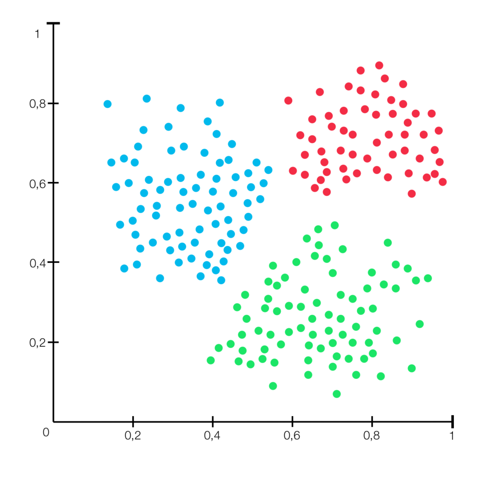
This type of clustering divides data points into a fixed number of pre-defined clusters. A popular example is K-Means clustering, which iteratively assigns data points to the nearest cluster centroid (mean) until a convergence criterion is met.

K-Means Clustering

K-means algorithm is iterative. First, define means called K value(k points).partitions a data set into clusters and randomly selected centroids(centre point). This process is repetitive until the cluster formed is homogeneous and the points in each cluster are close. The algorithm tries to maintain enough separability between these clusters. Due to the unsupervised nature, the clusters have no labels.

#import KMeans library from sklearn.cluster
from sklearn.cluster import KMeans
kmeans = KMeans(n_clusters=2) # want 2 cluster
kmeans.fit(X)

Full Code: Click Hear.

Hierarchical Clustering:

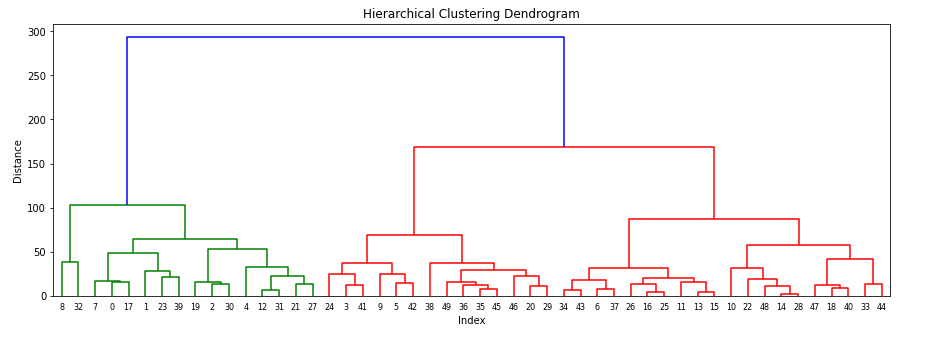
This approach builds a hierarchy of clusters, starting with individual data points and progressively merging them into larger clusters based on similarity. The resulting structure resembles a tree-like hierarchy (dendrogram).

Density-Based Clustering:

These algorithms identify clusters based on areas of high data density, separated by regions of low density. DBSCAN (Density-Based Spatial Clustering of Applications with Noise) is a well-known example, which can effectively handle clusters of arbitrary shapes and identify outliers.

Python Code Examples for Clustering Techniques

Let’s solidify our understanding with some code examples using popular Python libraries:

1. K-Means Clustering with scikit-learn:

from sklearn.cluster import KMeans

# Load your data (replace with your actual data)
X = ...

# Define the number of clusters (k)
n_clusters = 3

# Create a KMeans object
kmeans = KMeans(n_clusters=n_clusters, random_state=42)

# Fit the KMeans model to the data
kmeans.fit(X)

# Get the cluster labels for each data point
cluster_labels = kmeans.labels_

# Utilize the cluster labels for further analysis or visualization

This code snippet demonstrates performing K-Means clustering with scikit-learn. We define the number of desired clusters and create a KMeans object. The fit method trains the model on the data, and the labels_ attribute stores the cluster labels assigned to each data point. These labels can be used for further analysis or visualization tasks.

2. Hierarchical Clustering with scikit-learn:

from sklearn.cluster import AgglomerativeClustering

# Load your data (replace with your actual data)
X = ...

# Define the number of clusters (desired number of final clusters)
n_clusters = 3

# Create an AgglomerativeClustering object (using Ward's method)
ward_clustering = AgglomerativeClustering(n_clusters=n_clusters, linkage='ward')

# Fit the hierarchical clustering model to the data
ward_clustering.fit(X)

# Get the cluster labels for each data point
cluster_labels = ward_clustering.labels_

# Utilize the cluster labels for further analysis or visualization

This code example showcases hierarchical clustering using AgglomerativeClustering from scikit-learn. We specify the desired number of final clusters and create an object using Ward’s linkage method (a common agglomerative clustering approach). The fit method performs the clustering, and the labels_ attribute stores the cluster labels for each data point.

What is Linkage

Linkage is the criteria base on which distances between two clusters are compute: Single, Complete, Average.

• Single Linkage– The distance between two clusters is define as the shortest distance between two points in each cluster. 
• Complete Linkage – The distance between two clusters is define as the long distance between two points in each cluster. 
• Average Linkage – the distance between two clusters is define as the average distance between each point in one cluster to every other cluster.

#import AgglomerativeClustering from sklearn.cluster library 
from sklearn.cluster import AgglomerativeClustering 
#build Agglomerative Hierarchical Clustering
h_complete=AgglomerativeClustering(n_clusters=3,linkage='complete',affinity = "euclidean").fit(X)

Full Code: Click Here.

3. DBSCAN Clustering with scikit-learn:

from sklearn.cluster import DBSCAN

# Load your data (replace with your actual data)
X = ...

# Define the minimum number of points to form a cluster (min_samples)
# and the maximum distance between points to be considered in the same cluster (eps)
min_samples = 5
eps = 0.5

# Create a DBSCAN object
dbscan = DBSCAN(min_samples=min_samples, eps=eps, metric='euclidean')

# Fit the DBSCAN model to the data
dbscan.fit(X)

# Get the cluster labels for each data point (including -1 for noise points)
cluster_labels = dbscan.labels_

# Utilize the cluster labels and core samples for further analysis or visualization

# Optionally, get the indices of core samples
core_samples_mask = np.zeros_like(dbscan.labels_, dtype=bool)
core_samples_mask = dbscan.core_sample_indices_

# Print cluster labels for illustration
print("Cluster labels:")
print(cluster_labels)

# Print core samples for illustration (optional)
print("Core samples:")
print(core_samples_mask)

Explanation of Additions:

• Import numpy: This line imports the numpy library, which is used for creating the boolean mask for core samples.
• Metric argument: The metric argument in the DBSCAN object constructor specifies the distance metric used to calculate distances between data points. Here, we use the most common Euclidean distance metric.
• Core Sample Handling: The code snippet includes optional lines to get the core sample indices using dbscan.core_sample_indices_. You can utilize these indices to identify data points classified as core samples by the DBSCAN algorithm.
• Printing Results: The code now explicitly prints the cluster labels and core samples (if retrieved) for illustration purposes.

Remember to replace X with your actual data before running the code.

Considerations and Best Practices

Data Preprocessing: Clustering algorithms often perform better on preprocessed data. Techniques like normalization, scaling, and handling missing values can significantly impact the effectiveness of clustering.

Evaluation Metrics: There’s no single “golden standard” for evaluating clustering results. Consider metrics like silhouette score (measures how well data points are assigned to their clusters), Calinski-Harabasz index (compares the variance within clusters to the variance between clusters), and visualization techniques to assess the quality of your clusters.

The Art of Choosing K (for K-Means): The elbow method is a common technique to determine the optimal number of clusters for K-Means. It involves plotting the sum of squared errors (inertia) within clusters for different values of k and observing where the curve “elbows out,” indicating the optimal number of clusters.

Understanding Cluster Stability: It’s essential to assess the stability of your clusters, meaning how consistent the clustering results are with slight variations in the data. Techniques like silhouette analysis or running the clustering algorithm multiple times with different random states can help evaluate stability.

Dimensionality Reduction: For high-dimensional data, consider dimensionality reduction techniques like Principal Component Analysis (PCA) before clustering to improve efficiency and potentially enhance cluster separation.

Visualization: Visualization plays a crucial role in understanding clustering results. Techniques like scatter plots with color-coded clusters or dimensionality reduction for visualization with libraries like matplotlib or seaborn can be immensely helpful.

Advanced Techniques and Applications

The realm of clustering extends beyond the fundamental techniques discussed here. Here’s a glimpse into some advanced approaches:

• Spectral Clustering: This technique leverages spectral properties of a similarity matrix to group data points.
• Fuzzy Clustering: Unlike traditional clustering where each data point belongs to a single cluster, fuzzy clustering allows for partial membership in multiple clusters.
• Clustering with Constraints: Incorporate domain knowledge by specifying constraints on the clustering process, such as enforcing a minimum or maximum cluster size.

Clustering Applications:

• Customer Segmentation: Clustering customer data can help identify distinct customer groups with similar characteristics, enabling targeted marketing campaigns.
• Image Segmentation: Clustering techniques are use in image segmentation to group pixels with similar features, aiding in object recognition or image analysis.
• Document Clustering: Clustering documents base on their content can be use for topic modeling, information retrieval, and document organization.
• Anomaly Detection: Identifying data points that deviate significantly from their clusters can be indicative of anomalies or outliers, useful in fraud detection or system health monitoring.

Conclusion: Delving Deeper into the World of Clusters

Clustering in Python equips you with a powerful tool to uncover hidden structures within your data. By effectively applying clustering techniques, you can organize data into meaningful groups, leading to valuable insights. Remember, mastering clustering involves not only understanding the algorithms but also carefully selecting techniques based on your data and goals. Explore advanced clustering methods like spectral clustering or affinity propagation as you delve deeper into this fascinating domain. With your newfound knowledge, embark on a journey of uncovering the hidden landscapes within your data!