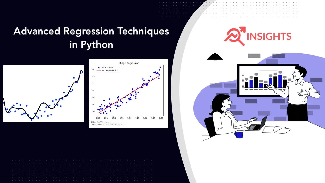
Have you ever wondered how Netflix predicts your next favorite show? Or how Amazon knows exactly what you want to buy? Advanced regression techniques in Python are behind these amazing feats. These powerful tools help data scientists extract insights from complex datasets. Let’s dive into the world of advanced regression and see how it’s shaping our digital landscape.
Why Advanced Regression Techniques Matter
Advanced regression goes beyond simple linear models. It handles complex relationships in data. These techniques can:
- Capture non-linear patterns
- Deal with high-dimensional data
- Handle interactions between variables
- Improve prediction accuracy
As a result, they’re invaluable in fields like finance, healthcare, and marketing.
Setting Up Your Python Environment
Before we start, let’s set up our Python environment. We’ll need these libraries:
- NumPy: For numerical operations
- Pandas: For data manipulation
- Scikit-learn: For machine learning models
- Matplotlib: For data visualization
Install them using pip:
pip install numpy pandas scikit-learn matplotlib
Polynomial Regression
Polynomial regression extends linear regression to capture non-linear relationships. It adds polynomial terms to the model.
from sklearn.preprocessing import PolynomialFeatures
from sklearn.linear_model import LinearRegression
from sklearn.pipeline import make_pipeline

degree = 3
polyreg = make_pipeline(PolynomialFeatures(degree), LinearRegression())
polyreg.fit(X, y)
This model can fit curved patterns in your data.
Ridge Regression
Ridge regression adds a penalty term to the linear regression cost function. This helps prevent overfitting.
from sklearn.linear_model import Ridge

ridge = Ridge(alpha=1.0)
ridge.fit(X, y)
The alpha parameter controls the strength of regularization.
Lasso Regression
Lasso regression also adds a penalty term. However, it can shrink some coefficients to zero, performing feature selection.
from sklearn.linear_model import Lasso

lasso = Lasso(alpha=1.0)
lasso.fit(X, y)
Lasso is useful when you have many features and want to identify the most important ones.
Elastic Net
Elastic Net combines Ridge and Lasso regularization. It provides a balance between the two approaches.
from sklearn.linear_model import ElasticNet

enet = ElasticNet(alpha=1.0, l1_ratio=0.5)
enet.fit(X, y)
The l1_ratio parameter controls the mix of Ridge and Lasso penalties.
Support Vector Regression (SVR)
SVR uses support vector machines for regression tasks. It’s effective for non-linear relationships.
from sklearn.svm import SVR

svr = SVR(kernel='rbf', C=1.0, epsilon=0.1)
svr.fit(X, y)
The kernel parameter defines the type of kernel used in the algorithm.
Decision Tree Regression
Decision trees split the data into subsets based on feature values. They can capture complex patterns.
from sklearn.tree import DecisionTreeRegressor

dt = DecisionTreeRegressor(max_depth=5)
dt.fit(X, y)
The max_depth parameter controls the complexity of the tree.
Random Forest Regression
Random Forest combines multiple decision trees. It often provides better performance than a single tree.
from sklearn.ensemble import RandomForestRegressor

rf = RandomForestRegressor(n_estimators=100, random_state=42)
rf.fit(X, y)
The n_estimators parameter sets the number of trees in the forest.
Gradient Boosting Regression
Gradient Boosting builds trees sequentially, with each tree correcting the errors of the previous ones.
from sklearn.ensemble import GradientBoostingRegressor

gb = GradientBoostingRegressor(n_estimators=100, learning_rate=0.1, max_depth=3)
gb.fit(X, y)
The learning_rate parameter controls how much each tree contributes to the final prediction.
XGBoost
XGBoost is an optimized implementation of gradient boosting. It’s known for its speed and performance.
from xgboost import XGBRegressor

xgb = XGBRegressor(n_estimators=100, learning_rate=0.1, max_depth=3)
xgb.fit(X, y)
XGBoost often performs well in machine learning competitions.
LightGBM
LightGBM is another gradient boosting framework. It’s designed for efficiency with large datasets.
from lightgbm import LGBMRegressor

lgbm = LGBMRegressor(n_estimators=100, learning_rate=0.1, max_depth=3)
lgbm.fit(X, y)
LightGBM uses a leaf-wise growth strategy, unlike the level-wise approach of traditional algorithms.
Neural Network Regression
Neural networks can model complex non-linear relationships. They’re versatile but may require more data.
from sklearn.neural_network import MLPRegressor

nn = MLPRegressor(hidden_layer_sizes=(100, 50), max_iter=500)
nn.fit(X, y)
The hidden_layer_sizes parameter defines the architecture of the network.
K-Nearest Neighbors Regression
K-Nearest Neighbors predicts based on the values of nearby points. It’s simple but can be effective.
from sklearn.neighbors import KNeighborsRegressor

knn = KNeighborsRegressor(n_neighbors=5)
knn.fit(X, y)
The n_neighbors parameter sets the number of neighbors to consider.
Gaussian Process Regression
Gaussian Process Regression provides probabilistic predictions. It’s useful when uncertainty estimates are needed.
from sklearn.gaussian_process import GaussianProcessRegressor

gpr = GaussianProcessRegressor()
gpr.fit(X, y)
This model can provide confidence intervals for its predictions.
Handling Categorical Variables
Many regression techniques require numerical inputs. We can handle categorical variables using encoding:
from sklearn.preprocessing import OneHotEncoder
from sklearn.compose import ColumnTransformer

categorical_features = ['category_column']
onehot = OneHotEncoder(sparse=False)

preprocessor = ColumnTransformer(
    transformers=[('onehot', onehot, categorical_features)],
    remainder='passthrough'
)

X_encoded = preprocessor.fit_transform(X)
This transforms categorical variables into numerical features.
Feature Scaling
Some models perform better with scaled features. We can use StandardScaler:
from sklearn.preprocessing import StandardScaler

scaler = StandardScaler()
X_scaled = scaler.fit_transform(X)
This scales features to have zero mean and unit variance.
Cross-Validation
Cross-validation helps assess model performance more reliably. We can use K-Fold cross-validation:
from sklearn.model_selection import cross_val_score

scores = cross_val_score(model, X, y, cv=5)
print("Mean score:", scores.mean())
This gives us a more robust estimate of model performance.
Hyperparameter Tuning
We can optimize model hyperparameters using grid search:
from sklearn.model_selection import GridSearchCV

param_grid = {'alpha': [0.1, 1.0, 10.0]}
grid_search = GridSearchCV(Ridge(), param_grid, cv=5)
grid_search.fit(X, y)

print("Best parameters:", grid_search.best_params_)
This helps find the best hyperparameters for our model.
Ensemble Methods
We can combine multiple models to improve performance:
from sklearn.ensemble import VotingRegressor

reg1 = RandomForestRegressor()
reg2 = GradientBoostingRegressor()
reg3 = LinearRegression()

ereg = VotingRegressor([('rf', reg1), ('gb', reg2), ('lr', reg3)])
ereg.fit(X, y)
This creates an ensemble of different models.
Interpreting Model Results
Understanding model predictions is crucial. For linear models, we can examine coefficients:
coefficients = pd.DataFrame({'feature': X.columns, 'coef': model.coef_})
print(coefficients.sort_values('coef', ascending=False))
For tree-based models, we can look at feature importances:
importances = pd.DataFrame({'feature': X.columns, 'importance': model.feature_importances_})
print(importances.sort_values('importance', ascending=False))
Conclusion
Advanced regression techniques in Python offer powerful tools for data analysis. From polynomial regression to ensemble methods, these techniques can handle a wide range of complex problems. By mastering these tools, you’ll be well-equipped to tackle challenging regression tasks in various fields.
Remember, no single technique is best for all problems. Experiment with different approaches and choose the one that works best for your specific dataset and problem. Happy modeling!
