What Is Forecasting?
Forecasting is a process of prediction or estimating the future based on past and present data. Example: how many passenger can we expect in a given flight?, weather forecasting, stock price forecasting.
Forecast means to contrive or scheme before hand; to arrange plan before execution.
What Is Time Series Forecasting?
Time Series is looking at data over time to forecast or predict what will happen in the next time period, based on patterns or re-occurring trends from previous time periods. History often repeats itself, so whatever events happened in the past, they are likely to happen again in the future.
The most common, basic example of a time series is seasonal sales revenue.Each year during the holidays, sales revenue goes up, and during off seasons, sales go down.
Time Series Assumptions
When Not Use Time Series?
- when the values are constant
- sales 500 coffee in the previous month. then this month also the sales number is almost the same that is 500. we wanted to predict the number of sales in the next month. now in such cases where the values are constant as in our case. the number of sales so 500 in the previous month and then in this month also. we have the same number and now we want to predict it for the next month. so in such cases where the values are constant time.
- When value can be represented using known functions for example the sine X
- if you have the x value you can get that value using by putting it in the function now you can apply time series analysis on this as well but there is no point because you can you could have got that value by putting it in the function itself.
When Use Time Series?
- data should be stationary
what is stationary data?
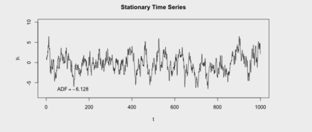
Time series has a particular behaviour over time, there is a very high probability that it will follow the same in the future. it’s call stationary.
Joint probability of a series does’t change over time. mean and variance remain constant over time. also no tend in series. known as strict stationary.

Constant mean, variance and auto covariance. Two time point t1 & t2. The covariance between Yt1 and Yt2 is the auto covariance known as Weak stationary process.
Auto(t1,t2) = Auto(t3,t4) = Auto(t5,t6)
Components of Time Series
Trend Component

in trend component, overall upward or downward pattern due to population, technology etc for several years duration. trend can be monthly, quarterly or yearly .
seasonal component

Regular pattern of up and down fluctuations due to weather, customs etc occurs within one year. Example: Passenger traffic during 24 hours, Seasonal Vegetable price.
irregular or random or Noise Component

Unsystematic Fluctuations Due to Random Variation or unforeseen events such as union strike, war for sort duration and non repeating.
# python Coding
#LINEAR
import statsmodels.formula.api as smf
linear_model = smf.ols('Ridership~t',data=Train).fit()
pred_linear =  pd.Series(linear_model.predict(pd.DataFrame(Test['t'])))
rmse_linear = np.sqrt(np.mean((np.array(Test['Ridership'])-np.array(pred_linear))**2))
rmse_linear
#Exponential
Exp = smf.ols('log_Rider~t',data=Train).fit()
pred_Exp = pd.Series(Exp.predict(pd.DataFrame(Test['t'])))
rmse_Exp = np.sqrt(np.mean((np.array(Test['Ridership'])-np.array(np.exp(pred_Exp)))**2))
rmse_Exp
#Quadratic
Quad = smf.ols('Ridership~t+t_squared',data=Train).fit()
pred_Quad = pd.Series(Quad.predict(Test[["t","t_squared"]]))
rmse_Quad = np.sqrt(np.mean((np.array(Test['Ridership'])-np.array(pred_Quad))**2))
rmse_Quad
#Additive seasonality
add_sea = smf.ols('Ridership~Jan+Feb+Mar+Apr+May+Jun+Jul+Aug+Sep+Oct+Nov',data=Train).fit()
pred_add_sea = pd.Series(add_sea.predict(Test[['Jan','Feb','Mar','Apr','May','Jun','Jul','Aug','Sep','Oct','Nov']]))
rmse_add_sea = np.sqrt(np.mean((np.array(Test['Ridership'])-np.array(pred_add_sea))**2))
rmse_add_sea
Full Python Code: Click Hear
# R Coding
# LINEAR MODEL
linear_model<-lm(Sales~t,data=train)
summary(linear_model)
linear_pred<-data.frame(predict(linear_model,interval='predict',newdata =test))
View(linear_pred)
rmse_linear<-sqrt(mean((test$Sales-linear_pred$fit)^2,na.rm = T))
rmse_linear
# Exponential
expo_model<-lm(log_Sales~t,data=train)
summary(expo_model)
expo_pred<-data.frame(predict(expo_model,interval='predict',newdata=test))
rmse_expo<-sqrt(mean((test$Sales-exp(expo_pred$fit))^2,na.rm = T))
rmse_expo
# Quadratic
Quad_model<-lm(Sales~t+t_square,data=train)
summary(Quad_model)
Quad_pred<-data.frame(predict(Quad_model,interval='predict',newdata=test))
rmse_Quad<-sqrt(mean((test$Sales-Quad_pred$fit)^2,na.rm=T))
rmse_Quad # 297.4067 and Adjusted R2 - 30.48%
# Additive Seasonality
sea_add_model<-lm(Sales~Jan+Feb+Mar+Apr+May+Jun+Jul+Aug+Sep+Oct+Nov+Dec,data=train)
summary(sea_add_model)
sea_add_pred<-data.frame(predict(sea_add_model,newdata=test,interval='predict'))
rmse_sea_add<-sqrt(mean((test$Sales-sea_add_pred$fit)^2,na.rm = T))
rmse_sea_add
Full R Code : Click Hear
ARIMA Model
ARIMA stands for Auto-Regressive Integrated Moving Average. ARIMA is basically the combination of two models that is AR And MA. AR model stands for auto regressive part an MA model stands for moving average. in simple word, AR is a separate model. MA is a separate model. what binds it together is the integration part that is indicated by I. AR is nothing but the correlation between the previous time period to the current. in MA, some kind of noise or irregularity attached in a time series so need to figure out that noise in fact. we need to average that out now whenever we try to average it out the cross and drop set of prison in that noise smoothen out and we can have average focused of that noise.
let’s take Example , you are standing at a time period t and there are previous time periods like (t-1) (t-2) (t-3) now if you find any correlation between (t-3)&t that called as auto regressive.
Arima need a three parameters: P, D, and Q. P stands for auto regressive, D for integrated (order of differentiation) and Q for moving average. p,d,q for non seasonal Arima Parameter and P,D And Q for seasonal.
ARIMA Model In R
#bulid Arima model
#p should be 0 based on ACF cut off
#q should be 1 or 2
(fit <- arima(log(AirPassengers), c(0, 1, 1),seasonal = list(order = c(0, 1, 1), period = 12)))
#Fit Model And predict the future 10 years
pred <- predict(fit, n.ahead = 10*12)
ts.plot(AirPassengers,2.718^pred$pred, log = "y", lty = c(1,3))
Full Code R : Click Hear
ARIMA Model In Python
# Import the library
from pmdarima.arima import auto_arima
# Ignore harmless warnings
import warnings
warnings.filterwarnings("ignore")
# Fit auto_arima function
stepwise_fit = auto_arima(airline['#Passengers'], start_p = 1, start_q = 1, max_p = 3, max_q = 3, m = 12, start_P = 0, seasonal = True, d = None, D = 1, trace = True,
error_action ='ignore', # we don't want to know if an order does not work
suppress_warnings = True, # we don't want convergence warnings
stepwise = True) # set to stepwise
# To print the summary
stepwise_fit.summary()
Python Full Code : Click Hear
